Friday, December 30, 2022

Short Takes: Bond Surprise and Sticking to a Plan

When people suggest topics for me to write about, more often than not I can point to an article I’ve already written, which is handy for me.  I doubt I’ll ever run out of thoughts on new topics, but it’s good to have a body of work to refer to.

Here are my posts for the past two weeks:

Car Companies Complaining about Interest Rates

RRSP Confusion


Searching for a Safe Withdrawal Rate: the Effect of Sampling Block Size

Here are some short takes and some weekend reading:


Ben Carlson
lists some things in the markets that surprised him this year.  The first thing is that stocks and bonds both went down double-digits.  Apparently, that’s never happened before.  I guess if you just look at the history of stock and bond returns, this outcome looks surprising.  However, when you look at the conditions we’ve come through, this was one among a handful of likely outcomes.  Bond markets were being artificially propped up, and the dam had to burst sometime.  As for stocks, the Shiller CAPE nearly reached 40.  We can’t know exactly when the next stock correction will happen, but the odds rise as the CAPE enters nosebleed territory.

Robb Engen sets a good example of sticking to his plan and making few trades despite a difficult 2022 for investors.

Wednesday, December 28, 2022

Searching for a Safe Withdrawal Rate: the Effect of Sampling Block Size

How much can we spend from a portfolio each year in retirement?  An early answer to this question came from William Bengen and became known as the 4% rule.  Recently, Ben Felix reported on research showing that it’s more sensible to use a 2.7% rule.  Here, I examine how a seemingly minor detail, the size of the sampling blocks of stock and bond returns, affects the final conclusion of the safe withdrawal percentage.  It turns out to make a significant difference.  In my usual style, I will try to make my explanations understandable to non-specialists.

The research

Bengen’s original 4% rule was based on U.S. stock and bond returns for Americans retiring between 1926 and 1976.  He determined that if these hypothetical retirees invested 50-75% in stocks and the rest in bonds, they could spend 4% of their portfolios in their first year of retirement and increase this dollar amount with inflation each year, and they wouldn’t run out of money within 30 years.

Researchers Anarkulova, Cederburg, O’Doherty, and Sias observed that U.S. markets were unusually good in the 20th century, and that foreign markets didn’t fare as well.  Further, there is no reason to believe that U.S. markets will continue to perform as well in the future.  They also observed that people often live longer in retirement than 30 years.  

Anarkulova et al. collected worldwide market data as well as mortality data, and found that the safe withdrawal rate (5% chance of running out of money) for 65-year olds who invest within their own countries is only 2.26%!  In follow-up communications with Felix, Cederburg reported that this increases to 2.7% for retirees who diversify their investments internationally.

Sampling block size

One of the challenges of creating a pattern of plausible future market returns is that we don’t have very much historical data.  A century may be a long time, but 100 data points of annual returns is a very small sample.  

Bengen used actual market data to see how 51 hypothetical retirees would have fared.  Anarkulova et al. used a method called bootstrapping.  They ran many simulations to generate possible market returns by choosing blocks of years randomly and stitching them together to fill a complete retirement.  

They chose the block sizes randomly (with a geometric distribution) with an average length of 10 years.  If the block sizes were exactly 10 years long, this means that the simulator would go to random places in the history of market returns and grab enough 10-year blocks to last a full retirement.  Then the simulator would test whether a retiree experiencing this fictitious return history would have run out of money at a given withdrawal rate.

In reality, the block sizes varied with the average being 10 years.  This average block size might seem like an insignificant detail, but it makes an important difference.  After going through the results of my own experiments, I’ll give an intuitive explanation of why the block size matters.

My contribution

I decided to examine how big a difference this block size makes to the safe withdrawal percentage.  Unfortunately, I don’t have the data set of market returns Anarkulova et al. used.  I chose to create a simpler setup designed to isolate the effect of sampling block size.  I also chose to use a fixed retirement length of 40 years rather than try to model mortality tables.

A minor technicality is that when I started a block of returns late in my dataset and needed a block extending beyond the end of the dataset, I wrapped around to the beginning of the dataset.  This isn’t ideal, but it is the same across all my experiments here, so it shouldn’t affect my goal to isolate the effect of sampling block size.

I obtained U.S. stock and bond returns going back to 1926.  Then I subtracted a fixed amount from all the samples.  I chose this fixed amount so that for a 40-year retirement, a portfolio 75% in stocks, and using a 10-year average sampling block size, the 95% safe withdrawal rate came to 2.7%.  The goal here was to use a data set that matches the Anarkulova et al. dataset in the sense that it gives the same safe withdrawal rate.  I used this dataset of reduced U.S. market returns for all my experiments.

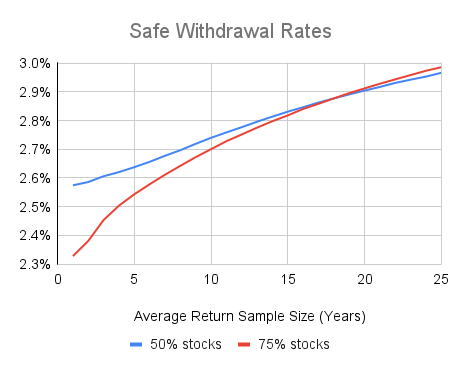
I then varied the average block size from 1 to 25 years, and simulated a billion retirements in each case to find the 95% safe withdrawal rate.  This first set of results was based on investing 75% in stocks.  I repeated this process for portfolios with only 50% in stocks.  The results are in the following chart.


The chart shows that the average sample size makes a significant difference.  For comparison, I also found the 100% safe withdrawal rate for the case where a herd of retirees each start their retirement in a different year of the available return data in the dataset.  In this case, block samples are unbroken (except for wrapping back to 1926 when necessary) and cover the whole retirement.  This 100% safe withdrawal rate was 3.07% for 75% stocks, and 3.09% for 50% stocks.  

I was mainly concerned with the gap between two cases: (1) the case similar to the Anarkulova et al. research where the average sampling block size is 10 years and we seek a 95% success probability, and (2) the 100% success rate for a herd of retirees case described above.  For 75% stock portfolios, this gap is 0.37%, and it is 0.32% for portfolios with 50% stocks.

In my opinion, it makes sense to add an estimate of this gap back onto the Anarkulova et al. 95% safe withdrawal rate of 2.7% to get a more reasonable estimate of the actual safe withdrawal rate.  I will explain my reasons for this after the following explanation of why sampling block sizes make a difference.

Why do sampling block sizes matter?

It is easier to understand why block size in the sampling process makes a difference if we consider a simpler case.  Suppose that we are simulating 40-year retirements by selecting two 20-year return histories from our dataset.

For the purposes of this discussion, let’s take all our 20-year return histories and order them from best to worst, and call the bottom 25% of them “poor.”

If we examine the poor 20-year return histories, we’ll find that, on average, stock valuations were above average at the start of the 20-year periods and below average at the end.  We’ll also find that investor sentiment about stocks will tend to be optimistic at the start and pessimistic at the end.  This won’t be true of all poor 20-year periods, but it will be true on average.

When the simulator chooses two poor periods in a row to build a hypothetical retirement, there will often be a disconnect in the middle.  Stock valuations will jump from low to high and investor sentiment from low to high instantaneously, without any corresponding instantaneous change in stock prices.  This can’t happen in the real world.

Each time we randomly-select a sample from the dataset, there is a 1 in 4 chance it will be poor.  The probability of choosing two poor samples when building a 40-year retirement is then 1 in 16.  However, in the real world, the probability of a poor 20-year period being followed by another poor period is lower than 1 in 4.  The probability of a 40-year retirement in the real world consisting of two poor 20-year periods is less than 1 in 16.

Of course, by similar reasoning, the simulator will also produce too many hypothetical retirements with two good 20-year periods.  So, we might ask whether all this will balance out.  The answer is no, because we are looking for the withdrawal rate that will fail only 5% of the time.

Good outcomes from the simulator are largely irrelevant.  We are looking for the retirement outcome that is worse than 95% of all other outcomes.  When the simulator produces too many doubly-poor outcomes, it drives down this 95% point.  The result is an overly pessimistic safe withdrawal rate.

In the more complex case of the simulators discussed here, we are joining return histories of varying lengths, but the problem with disconnects in stock valuations and investor sentiment at the join points is the same.  The more join points we have, the more disconnects we create.  So, the lower the average return sample length, the lower the safe withdrawal rate result.  This is what we saw in the charts above.

In more mathematical terms, the autocorrelations in actual stock prices result in poor periods tending to be followed by above-average periods, and vice-versa. This is called mean reversion.  When we select samples from the return dataset and join them together, we partially destroy this mean reversion.  The shorter the return samples, the more mean reversion we remove.

Anarkulova et al. selected fairly long samples from their dataset (a decade on average) to try to preserve mean reversion.  This helped somewhat, but mean reversion exists on the decade level as well, and choosing 10-year blocks of returns destroys mean reversion between the decades.

What is the remedy?

Anarkulova et al. aren’t misguided in the methods they use.  There just isn’t enough available historical return data to run this type of experiment without getting creative.  If we had a million years of actual stock returns rather than just a century or so, it would be much easier to determine safe withdrawal rates.

However, we can’t just ignore the problem of properly preserving mean reversion.  My best guess is that we need to take the roughly 0.3% gap I observed between Anarkulova et al. approach and the “herd of retirees” approach (described earlier) and add it to the 2.7% withdrawal rate calculated by Anarkulova et al.  This gives a base withdrawal rate of 3.0%.  Fans of the 4% rule will still find this result disappointingly low, but I believe it is reasonable.

From there a retiree can adjust for other factors.  For example, we need to deduct about half the MERs we pay.  We also need to spend less if we retire before age 65, and can spend more if we retire after age 65.  Another adjustment is that we can withdraw more initially if we are prepared to reduce spending if markets disappoint rather than blindly spend our portfolios down to zero as Bengen’s original 4% rule would have us do.  Another adjustment for me is that my total costs (including foreign withholding taxes) on investments outside Canada are lower than the 0.5% assumed by Anarkulova et al.  We can make further adjustments if our mortality probabilities are different from the average.

Safe withdrawal rates are a complex area where most of what we read is biased toward telling us we can spend more.  Anarkulova et al. used reasonable historical returns and mortality tables to provide an important message that safe withdrawal rates are lower than we may think.  However, as I’ve argued here, I think they are too pessimistic.

Friday, December 23, 2022

RRSP Confusion

Recently, I was helping a young person with his first ever RRSP contribution, and this made me think it’s a good time to explain a confusing part of the RRSP rules: contributions in January and February.  Reader Chris Reed understands this topic well, and he suggested that an explanation would be useful for the upcoming RRSP season.

Contributions and deductions are separate steps

We tend to think of RRSP contributions and deductions as parts of the same set of steps, but they don’t have to be.  For example, if you have RRSP room, you can make a contribution now and take the corresponding tax deduction off your income in some future year.

An important note from Brin in the comment section below: “you have to *report* the contribution when filing your taxes even if you’ve decided not to use the deduction until later. It’s not like charitable donations, where if you’re saving a donation credit for next year you don’t say anything about it this year.”

Most of the time, people take the deductions off their incomes in the same year they made their contributions, but they don’t have to.  Waiting to take the deduction can make sense in certain circumstances.  For example, suppose you get a $20,000 inheritance in a year when your income is low.  You might choose to make an RRSP contribution now, and take the tax deduction in a future year when your marginal tax rate is higher, so that you’ll get a bigger tax refund.

RRSP contribution room is based on the calendar year


Each year you are granted new RRSP contribution room based on your previous year’s tax filing.  This amount is equal to 18% of your prior year’s wages (up to a maximum and subject to reductions if you made pension contributions).  You can contribute this amount to your RRSP anytime starting January 1.

Many people think that the “RRSP year” runs from March to the following February, and that you have to wait until March to make an RRSP contribution for the new year.  This isn’t true.  If you have new 2023 RRSP contribution room coming to you, you can make the contribution in January if you like.  It’s when you take the RRSP tax deduction that there are special rules for the first 60 days of the year.  I’ll explain that further below.

One complication with using new RRSP contribution room in January or February is that you won’t have your notice of assessment yet to tell you the amount of room you have.  However, if you can calculate this amount yourself, you’re free to use the room at the start of the year.

If you’re waiting for CRA to calculate your new RRSP room for you, Chris Reed suggests that you “use the Contribution Room stated on your Notice of Assessment after filing your tax return, instead of your [CRA My Account] webpage.  That webpage often has errors.”

Taking RRSP deductions


To be allowed to take an RRSP deduction for the 2022 taxation year, you have to satisfy the following  two requirements.  Firstly, you must have made a contribution based on RRSP room for 2022 or an earlier year.  Secondly, you must have made the contribution sometime before 60 days after 2022 December 31.  Some examples will help to illustrate these requirements.

Suppose you made a contribution in 2021 that was part of your available 2021 room, but you didn’t take the deduction on your 2021 taxes.  Then you can take the deduction on your 2022 taxes.

Suppose you used up all your RRSP room and deductions in 2021, and you have $10,000 of room for 2022.  Suppose further that you will get another $15,000 of room for 2023.  You are allowed to make an RRSP contribution of $25,000 in January 2023.  However, you will only be able to deduct $10,000 from your income on your 2022 taxes.  The remaining $15,000 deduction will have to wait for your 2023 taxes (or a later year if you prefer).

Early birds who use their new 2023 contribution room in January or February 2023 might become nervous when filing their 2022 income taxes a month or two later when they discover that they can’t take the RRSP deduction right away.  They might think they’ve over-contributed.  They haven’t.  They’re just way ahead of all the people making 2022 contributions just under the wire.  They have to wait until the 2023 taxation year to take the deduction.

Monday, December 19, 2022

Car Companies Complaining about Interest Rates

I don’t often have much to say about macroeconomic issues, but an article “sounding the alarm” about how interest rate increases are affecting car companies drew a reaction.

“Aggressively raising interest rates has helped create an untenable situation in car financing.”

Good.  Financing a car is usually a mistake for the consumer.  When consumers’ credit is so bad that they can’t even get a car loan, it’s even clearer that they shouldn’t buy the car.

“The auto sector is one of the victims of the aggressive interest rate hikes.”

Ridiculously low interest rates have allowed car companies to inflate prices and sell ever more cars to people who can’t really afford them.  The fact that the party is ending doesn’t make car companies victims.  Conditions are just slowly getting back to normal.

“Rising interest rates will make consumers reevaluate their decisions before quickly jumping into a car loan.”

Good.  It’s sad when people bury their financial future by buying an expensive vehicle they can’t really afford.  If you’ve got the money, go ahead.  If not, consider a cheaper vehicle or other means of transportation.

“The average annual percentage rate (APR) for financing a new vehicle purchase climbed to 6.3% in October 2022, compared to 4.2% in October 2021, the highest new vehicle APR since April 2019.”

Interest rates are just getting back to a normal range.  The rates we’ve seen in recent years were unsustainably low.  Portraying today’s rates as excessively high is misleading.

“The last time interest rates were this high, consumers could at least rely on lower vehicle prices.”

One way to return to stability would be for central banks to lower interest rates again.  A better way is for car companies to lower their prices.

“Monetary policy continues to worsen the situation in the automobile industry, and has created a crisis that could explode in 2023.”

If we get an explosion of defaults on auto loans, I have some sympathy for unsophisticated buyers who didn’t understand the risks they were taking, but for the most part, reckless consumers and lenders deserve each other.

There are reasonable ways to use debt in your life, but buying a far more expensive vehicle than you need is not one of them.

Friday, December 16, 2022

Short Takes: U.S. Equity ETFs, Index Investing Advantage, and more

There’s a whole world of retired people who play sports that I didn’t know existed until the last few years.  As I aged and was trying to compete with much younger athletes, I often wondered how much longer I could keep going.  A common mindset among older players is that they’ll have to give it up sometime, probably soon.  However, when I play sports with people my age and older, I see that I can keep going as long as I can stay healthy enough.

Rather than focusing on how much physical ability I’ve lost, I can focus on finding people who play at roughly the same level I do.  This has increased my motivation to do targeted exercise to keep my body healthy enough to play sports.  You’d think that staying healthy and strong would be motivation enough, but I find the deadline of completing rehab before an upcoming sports season much more motivating.

Here are some short takes and some weekend reading:

Justin Bender compares U.S. stock ETFs domiciled in Canada (e.g., VUN) to those in the U.S. (e.g., VTI).  He takes into account differences in currency exchange costs and foreign withholding taxes in different types of accounts.  This motivates the need to use Norbert’s Gambit for currency exchanges when using U.S.-domiciled ETFs.

Andrew Hallam presents evidence that “Over a period of 35 years, index fund investors earn 100 percent more money than those who buy actively managed funds.”

Robb Engen at Boomer and Echo evaluates his 2022 financial goals and lays out new ones for 2023.  I like that he sets targets for things he can control, such as how much he will save in various accounts from his income.  He doesn’t set targets for things he can’t control, such as investment returns, the price he’ll get when selling his house, or his overall net worth.  For others trying to follow Robb’s lead, it’s important not to run up debts on credit cards, lines of credit or elsewhere to meet savings targets.  If savings targets prove unrealistic, it’s better to re-evaluate savings plans than it is to bury yourself in debt.

Friday, December 2, 2022

Short Takes: Bond Debacle, FTX Debacle, and more

It’s no secret that bonds got crushed this year as interest rates rose.  Rob Carrick went so far as to say “Given how absurdly low rates were in 2020 and 2021, your adviser should have seen the events of 2022 [the bond crash] coming.”  I agree in the sense that the bond crash was predictable, but its exact timing was not.  I explained the problem with long-term bonds back when there was still time to avoid the losses.

It’s important to be clear that I was not making a bond market prediction.  What was certain was that long-term bonds purchased in 2020 were going to perform very poorly over their lifetimes.  The exact timing of bond losses was not knowable with any certainty.  The tight coupling between interest rates and bond returns is what made it possible to see the brewing problems; this isn’t possible with stocks.

I’ve seen a few attempts by financial advisors to justify their failure to act for their clients by talking about how if you blend poor long-term bond returns with present and future short-term bonds returns, the blend isn’t too bad.  This is like tossing some sawdust into your soup.  The blend may be tolerable, but why include the sawdust?

Many advisors just look at annual bond returns and see their unpredictability as similar to stock returns, but this isn’t true.  Bond yields tell you exactly what average return you’ll get over the life of the bond.  This is true whether you own that bond on its own or blended into a fund.

The bond debacle wasn’t just predictable, it was certain to happen.

Here are my posts for the past two weeks:


When Small Fees Equate to High Interest Rates

Quit: The Power of Knowing When to Walk Away


Here are some short takes and some weekend reading:

Adam M. Grossman clearly explains what happened at FTX and the warning signs that investors ignored.

Jackson, Ling, and Naranjo show “evidence that private equity (PE) fund managers manipulate returns to cater to their investors.”  Some private equity investors get “phony happiness” from “overstated and smoothed interim returns.”

Tom Bradley at Steadyhand was inducted into the Investment Industry of Canada’s Hall of Fame.  His speech reveals what we’ve known about him for a long time: that he cares about his clients.

The Blunt Bean Counter
explains some of the subtleties of the Principal Residence Exemption (PRE).