
Searching for a Safe Withdrawal Rate: the Effect of Sampling Block Size
How much can we spend from a portfolio each year in retirement? An early answer to this question came from William Bengen and became known as the 4% rule. Recently, Ben Felix reported on research showing that it’s more sensible to use a 2.7% rule. Here, I examine how a seemingly minor detail, the size of the sampling blocks of stock and bond returns, affects the final conclusion of the safe withdrawal percentage. It turns out to make a significant difference. In my usual style, I will try to make my explanations understandable to non-specialists.
The research
Bengen’s original 4% rule was based on U.S. stock and bond returns for Americans retiring between 1926 and 1976. He determined that if these hypothetical retirees invested 50-75% in stocks and the rest in bonds, they could spend 4% of their portfolios in their first year of retirement and increase this dollar amount with inflation each year, and they wouldn’t run out of money within 30 years.
Researchers Anarkulova, Cederburg, O’Doherty, and Sias observed that U.S. markets were unusually good in the 20th century, and that foreign markets didn’t fare as well. Further, there is no reason to believe that U.S. markets will continue to perform as well in the future. They also observed that people often live longer in retirement than 30 years.
Anarkulova et al. collected worldwide market data as well as mortality data, and found that the safe withdrawal rate (5% chance of running out of money) for 65-year olds who invest within their own countries is only 2.26%! In follow-up communications with Felix, Cederburg reported that this increases to 2.7% for retirees who diversify their investments internationally.
Sampling block size
One of the challenges of creating a pattern of plausible future market returns is that we don’t have very much historical data. A century may be a long time, but 100 data points of annual returns is a very small sample.
Bengen used actual market data to see how 51 hypothetical retirees would have fared. Anarkulova et al. used a method called bootstrapping. They ran many simulations to generate possible market returns by choosing blocks of years randomly and stitching them together to fill a complete retirement.
They chose the block sizes randomly (with a geometric distribution) with an average length of 10 years. If the block sizes were exactly 10 years long, this means that the simulator would go to random places in the history of market returns and grab enough 10-year blocks to last a full retirement. Then the simulator would test whether a retiree experiencing this fictitious return history would have run out of money at a given withdrawal rate.
In reality, the block sizes varied with the average being 10 years. This average block size might seem like an insignificant detail, but it makes an important difference. After going through the results of my own experiments, I’ll give an intuitive explanation of why the block size matters.
My contribution
I decided to examine how big a difference this block size makes to the safe withdrawal percentage. Unfortunately, I don’t have the data set of market returns Anarkulova et al. used. I chose to create a simpler setup designed to isolate the effect of sampling block size. I also chose to use a fixed retirement length of 40 years rather than try to model mortality tables.
A minor technicality is that when I started a block of returns late in my dataset and needed a block extending beyond the end of the dataset, I wrapped around to the beginning of the dataset. This isn’t ideal, but it is the same across all my experiments here, so it shouldn’t affect my goal to isolate the effect of sampling block size.
I obtained U.S. stock and bond returns going back to 1926. Then I subtracted a fixed amount from all the samples. I chose this fixed amount so that for a 40-year retirement, a portfolio 75% in stocks, and using a 10-year average sampling block size, the 95% safe withdrawal rate came to 2.7%. The goal here was to use a data set that matches the Anarkulova et al. dataset in the sense that it gives the same safe withdrawal rate. I used this dataset of reduced U.S. market returns for all my experiments.
I then varied the average block size from 1 to 25 years, and simulated a billion retirements in each case to find the 95% safe withdrawal rate. This first set of results was based on investing 75% in stocks. I repeated this process for portfolios with only 50% in stocks. The results are in the following chart.
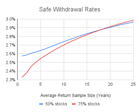
The chart shows that the average sample size makes a significant difference. For comparison, I also found the 100% safe withdrawal rate for the case where a herd of retirees each start their retirement in a different year of the available return data in the dataset. In this case, block samples are unbroken (except for wrapping back to 1926 when necessary) and cover the whole retirement. This 100% safe withdrawal rate was 3.07% for 75% stocks, and 3.09% for 50% stocks.
I was mainly concerned with the gap between two cases: (1) the case similar to the Anarkulova et al. research where the average sampling block size is 10 years and we seek a 95% success probability, and (2) the 100% success rate for a herd of retirees case described above. For 75% stock portfolios, this gap is 0.37%, and it is 0.32% for portfolios with 50% stocks.
In my opinion, it makes sense to add an estimate of this gap back onto the Anarkulova et al. 95% safe withdrawal rate of 2.7% to get a more reasonable estimate of the actual safe withdrawal rate. I will explain my reasons for this after the following explanation of why sampling block sizes make a difference.
Why do sampling block sizes matter?
It is easier to understand why block size in the sampling process makes a difference if we consider a simpler case. Suppose that we are simulating 40-year retirements by selecting two 20-year return histories from our dataset.
For the purposes of this discussion, let’s take all our 20-year return histories and order them from best to worst, and call the bottom 25% of them “poor.”
If we examine the poor 20-year return histories, we’ll find that, on average, stock valuations were above average at the start of the 20-year periods and below average at the end. We’ll also find that investor sentiment about stocks will tend to be optimistic at the start and pessimistic at the end. This won’t be true of all poor 20-year periods, but it will be true on average.
When the simulator chooses two poor periods in a row to build a hypothetical retirement, there will often be a disconnect in the middle. Stock valuations will jump from low to high and investor sentiment from low to high instantaneously, without any corresponding instantaneous change in stock prices. This can’t happen in the real world.
Each time we randomly-select a sample from the dataset, there is a 1 in 4 chance it will be poor. The probability of choosing two poor samples when building a 40-year retirement is then 1 in 16. However, in the real world, the probability of a poor 20-year period being followed by another poor period is lower than 1 in 4. The probability of a 40-year retirement in the real world consisting of two poor 20-year periods is less than 1 in 16.
Of course, by similar reasoning, the simulator will also produce too many hypothetical retirements with two good 20-year periods. So, we might ask whether all this will balance out. The answer is no, because we are looking for the withdrawal rate that will fail only 5% of the time.
Good outcomes from the simulator are largely irrelevant. We are looking for the retirement outcome that is worse than 95% of all other outcomes. When the simulator produces too many doubly-poor outcomes, it drives down this 95% point. The result is an overly pessimistic safe withdrawal rate.
In the more complex case of the simulators discussed here, we are joining return histories of varying lengths, but the problem with disconnects in stock valuations and investor sentiment at the join points is the same. The more join points we have, the more disconnects we create. So, the lower the average return sample length, the lower the safe withdrawal rate result. This is what we saw in the charts above.
In more mathematical terms, the autocorrelations in actual stock prices result in poor periods tending to be followed by above-average periods, and vice-versa. This is called mean reversion. When we select samples from the return dataset and join them together, we partially destroy this mean reversion. The shorter the return samples, the more mean reversion we remove.
Anarkulova et al. selected fairly long samples from their dataset (a decade on average) to try to preserve mean reversion. This helped somewhat, but mean reversion exists on the decade level as well, and choosing 10-year blocks of returns destroys mean reversion between the decades.
What is the remedy?
Anarkulova et al. aren’t misguided in the methods they use. There just isn’t enough available historical return data to run this type of experiment without getting creative. If we had a million years of actual stock returns rather than just a century or so, it would be much easier to determine safe withdrawal rates.
However, we can’t just ignore the problem of properly preserving mean reversion. My best guess is that we need to take the roughly 0.3% gap I observed between Anarkulova et al. approach and the “herd of retirees” approach (described earlier) and add it to the 2.7% withdrawal rate calculated by Anarkulova et al. This gives a base withdrawal rate of 3.0%. Fans of the 4% rule will still find this result disappointingly low, but I believe it is reasonable.
From there a retiree can adjust for other factors. For example, we need to deduct about half the MERs we pay. We also need to spend less if we retire before age 65, and can spend more if we retire after age 65. Another adjustment is that we can withdraw more initially if we are prepared to reduce spending if markets disappoint rather than blindly spend our portfolios down to zero as Bengen’s original 4% rule would have us do. Another adjustment for me is that my total costs (including foreign withholding taxes) on investments outside Canada are lower than the 0.5% assumed by Anarkulova et al. We can make further adjustments if our mortality probabilities are different from the average.
Safe withdrawal rates are a complex area where most of what we read is biased toward telling us we can spend more. Anarkulova et al. used reasonable historical returns and mortality tables to provide an important message that safe withdrawal rates are lower than we may think. However, as I’ve argued here, I think they are too pessimistic.
3% or so is all well and good for living off the investments alone, but CPP/OAS should push that number up by a fair bit, too.
ReplyDeleteWhat you say is true if you haven't begun CPP and OAS yet. However, once they start, the amount you can safely pull from your portfolio is 3% (with the adjustments I mentioned near the end of the article). Before CPP and OAS begin, but after retirement starts, you can make an additional portfolio withdrawal for the purpose of matching future CPP and OAS payments.
DeleteI always struggle with the Safe Withdrawal Rules / Variable Withdrawal Rules. I feel like it's completely "safe" for me to only withdraw my dividends / distributions. Currently, my average yield is 6.47% - but of course when the market rebounds it will be more like 5.2%, or something like that. That won't mean I will withdraw any more, or any less - but can't I consider this "safe"? Am I missing something when it comes to my plan to only use my dividends in retirement?
ReplyDeleteIt's of course "safe" to only spend dividends, but you'll die with a huge amount of money in the bank. You could be spending more and drawing down the capital as you go along (as long as you are certain to not exhaust it before death). Or alternatively, you could spend the same amount, but retire sooner, with less capital built up.
DeleteHi James,
DeleteWhen yields are this high, it can mean that the market thinks that this company's dividend is unsustainable, and that the dividend and stock price will come down (or fail to grow with inflation). Hard to know in any particular company's case.
Excellent analysis, Michael. So now we have the “3% Rule”. As per an earlier reader’s comment, for most retirees, during the 30-year “Rule” window they will be drawing CPP, OAS, and some will have DB pensions too. Bringing in two more variables i.e., amount of other income (% of desired income) and how early it commences in the retirement, could be more meaningful to many. Extremes are if this other income starts at day one of the retirement and covers 100% of the desired income, then the safe withdrawal rate is 100%. If, however, the other income starts at year 30, then, as we know from your analysis, the safe withdrawal rate is 3%. I don’t recall having seen a chart or table that combines a withdrawal Rule with other income, but I do think it would provide a useful guide to many. Perhaps this could be the subject for a future post.
ReplyDeleteHi Bob,
DeleteI think you are defining "safe withdrawal rate" differently from how I did in my article. It is the largest percentage you can draw from your portfolio in the first year such that if you increase this dollar amount of withdrawal by inflation each year, you are very likely to not run out of money while you're still alive. So, the safe withdrawal percentage can never be 100%.
If you are going to have future cash flows or pensions starting in the future, this can complicate the analysis. I wrote an article about this that points to a paper I wrote that explains how I do the calculations:
https://www.michaeljamesonmoney.com/2020/05/calculating-my-retirement-glidepath.html
The “return to the mean” claim seems intuitively true but also in direct contradiction to the Random Walk theory. And intuition is likely a poor basis for investing.
ReplyDeleteGood point about 100 years’ worth of data being too short of a period to predict 40 years’ worth of returns with “95% confidence”. However you slice it, we have a problem. And that’s before we try to align market condition to what’s in front of us (fiat money, QE/QT cycles, changes in how inflation target is pursued by CBs, etc)
Sadly, theory is often a poor basis for investing as well (except when it isn't :-).
DeleteHow have you dealt with the emotional side of your withdrawal rate?
ReplyDeleteI'm still in my accumulation phase and seeing my RRSP and TFSA combined pass milestones of 50k, 100k etc has made me feel proud and like I'm on track. Crossing 50k saving made me feel incredibly proud as it was a years net salary at the time.
But what does that feel like on the other side when you drop below a milestone? Lets say from 500k to 499k? Was it a gut punch that made you double check your withdrawal rate and spending? Or were you proud of having saved for so long that you now get to deploy those funds? Did it affect your significant other differently or did you have conversations ahead of time to smooth that transition of accumulation to spending phase?
When your portfolio gets much larger, the daily and monthly swings in its value swamp the size of new contributions or withdrawals. So, you don't really see a single transition from $500k to $499k. Any anxiety tends to come from seeing your portfolio drop due to market losses. While it's true that withdrawals contribute to that drop, they are less visible.
DeleteAs for my own experience, I was lucky enough to get the upside of order-of-returns risk. I retired in mid-2017 into the wave of an ongoing bull market. Even with the more recent market declines, I'm still significantly above the portfolio size I had at retirement. So, my anxiety level due to declining funds is largely untested. However, I never got stressed during any of the large market declines during my investment years.
Another great analysis, Michael. Interestingly enough, in his original paper, Bengen showed that a 3% inflation-adjusted withdrawal never depleted a portfolio (e.g., I think he use 50 years in his analysis). Although this was early analysis and bias towards US data, it remains a pretty reasonable guideline to use with global diversification. In reality, nothing will ever be 100%, because circumstances change and our assumptions are based on "best guesses" that are based on historical circumstances. In order to have a reasonable chance of never running out of money, use a "as conservative as possible withdrawal rate" and be prepared to make further adjustments (e.g., like temporary part time work or a side hustle as required ). The down side is that you'll likely die with too much money but you won't have sleepless nights worrying that you'll run out of money.
ReplyDeleteIn my case, I have a spreadsheet that tells me how much I can spend safely each month, but because of the long bull market, that amount exceeds my actual spending by a wide margin. So, my plan is to pass the excess to my kids as they demonstrate they can handle it. Either that or convince my wife we need to buy a second home on the water somewhere warm.
DeleteInteresting analysis. One issue I have always had with analysis using Monte Carlo or bootstrap (with or without replacement) simulations is that they ignore the autocorrelation that tends to occur, which is no guarantee. Block bootstrap overcomes that to a degree but as your analysis points out, the block size still has a significant impact.
ReplyDeleteWhile the past is no guarantee of the future, it does provide some indication of the range and bounds that one can expect. e.g. I don't think we have ever experienced double digit down years for 10 years in a row and I consider that unlikely, but that could happen with plain bootstrap or Monte Carlo.
I find the attempts to maintain autocorrelation using block bootstrap admirable, but I think mean reversion on the scale of decades is more important for buy-and-hold investors than short-term autocorrelation.
DeleteI appreciate Michael's review that steers us back to a more realistic and probable outcome. Once again, this plays out well for the financial planning firms, that place fear and doubt in our minds that a 3% SWR is now considered risky and not safe. Unfortunately, we can't outright say that they are wrong that because they use assumptions in their analysis. However, it's also important to understand that we can make assumptions as pessimistic as required to achieve a desired outcome. For instance, next year, new analysis will state that the new SWR be will be 2 % based on new assumptions that are often not very relatable to real life scenarios. To the best of my knowledge, a 3% SWR has never failed historically for a diversified portfolio with a higher stock to bond allocation! Nothing will ever be 100% safe but hedging your bets on a diversified portfolio with using a 3% SWR is likely as safe as it gets.
ReplyDeleteI don't have a lot of experience with financial planning firms, but I've seen a lot more advice suggesting 6-8% is safe than saying 3% isn't safe. The low figures seem to come mainly from academia.
DeleteWilliam J. Bernstein says “Below the age of 65, a 2% spending rate is bulletproof, 3% is probably safe, and 4% is taking chances. Above 5%, you’re taking an increasingly serious risk of dying poor. (For each five years above 65, add perhaps half a percentage point to those numbers.)”
Mike, I know this would be harder to compare but would you consider real estate income a better bet than equities and bonds considering that 3% is now just relatively safe. Assuming you own the rental properties free and clear ( like a stock portfolio) and in equivalent proportions.
DeleteAn important thing to remember about safe withdrawal rates (SWRs) is that retirees who are prepared to cut spending somewhat if necessary can spend more initially. If you're so inflexible that you will spend the same dollar amount every year (adjusted for inflation) no matter what happens to your portfolio, then you'd better start with at most 3%. However, if you're prepared to adjust as necessary, then 4% can be perfectly reasonable.
DeleteI don't see how owning rental properties can compare with stocks without using leverage, which adds considerable risk.
Michael,
DeleteA 3 million dollar portfolio invested stock/bond at a 3% SWR would provide about $90K, or 4 residential rental properties (~$750K each) would provide a "net annual" income of about $90K after all expenses, wouldn't the properties have the advantage here because of the rental income is net income? The properties and the rental income would also increase over time just like the stock/bond portfolio?
As I explained earlier, a 4% withdrawal rate is quite safe for a retiree willing to cut expenses if necessary, and the likely outcome is future withdrawals rising faster than inflation. Another thing to consider is that a stock/bond portfolio gives passive income, while rental properties come with the job of being a landlord.
Delete